physics – Datamuncher

Prolog

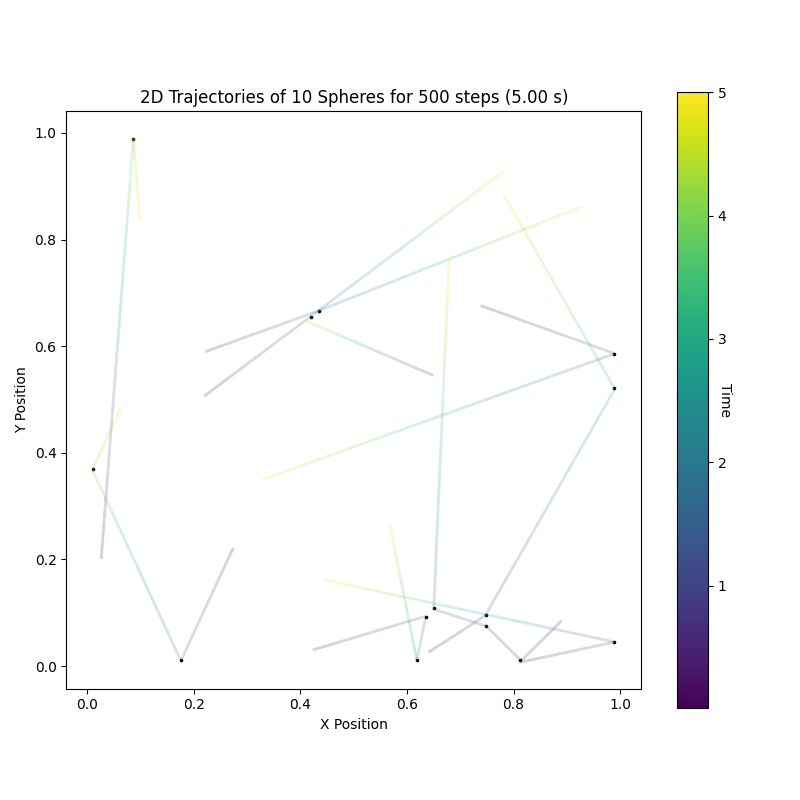
After I’ve recently been working on getting the dynamics simulation of hard spheres right, see my previous blog post, I was curious about color coding neighborhood symmetries. To see if my small simulations are already sufficient to see some sort of systematic change. Like can we see “melting” or “crystallization”? 🙂

Turns out yes, for a pretty animation see below. 🙂

You may think this is all settled and researchers have long moved on and everything is understood, spelled out in simple language, organized and filed away for easy grokking. But then you, as I was, would be mistaken. Study of hard spheres seems actually still a matter of ongoing research. There were even experiments done on the space shuttle in 2001, to study the transition between “liquid” and “solid” states (if you are interested in the general concept of “phases” and their transitions, I recommend this wiki page 🙂 ). And more definitive data on liquid-hexatic and hexatic-crystal transition was only collected in 2017. For what hexatic phases are see this wiki page.

Measuring symmetry

So I started researching a bit into how to measure “symmetries”. Various measures could come to mind, but given that hard spheres have been the prime model in statistical mechanics to study many body systems, there ought to be some I can use that have proven useful. If you want to research as well I recommend using the term “bond order parameters”.

I’ve settled on the following

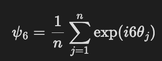
using all 6 nearest neighbors of a hard sphere. So the algorithm is like this:

pick a sphere
compute the distance vectors to all other spheres
compute the lengths of the distance vectors
pick the 6 smallest ones
for each distance vector take its x and y value to compute the angle theta = arctan(y,x)
multiply each angle with 6 and the imaginary unit “i”
exponentiate all values
compute the mean
repeat for the next sphere

and voila you’ve got psi-6 for all your spheres. For me it was most practical to use the absolute value of psi-6.

Visualizing melting

So how could we see “melting” of hard spheres?

By stacking them in a hexagonal grid and then running our molecular dynamics simulation. Easy! This then looks like this

The color scale varies from deep blue = far away from hexagonal order to deep red = perfect hexagonal order.

You may be wondering why the spheres escape upwards and to the right. That’s because I intentionally left some room between the outermost spheres and the simulation box, to encourage things to happen. Because by definition hard spheres don’t have any attractive forces between them they’ll want to fly away.

How to do it yourself

Interested in the code or in how I created the visualization?

I’ve put the code for the above on github for you to check out: https://github.com/eschmidt42/hardspheres-2d/tree/main

You can also install the simulation via uvx and run it from the command line via

uvx --from hardspheres-2d hardspheres2d --help

The visualisation was done using ovito. Scouring the web it just seemed the easiest tool for what I wanted to do. It also has a python package, but I didn’t get done with it what I wanted here. The basic free version of ovito is sufficient for the needs I had as well.

If you just want to dump the molecular dynamics snapshots generated with the above simulation, you can download https://github.com/eschmidt42/hardspheres-2d/blob/d6ea22740fcbf07c2b4d29d88fdc8c2a7f4271ca/hardspheres-hexagon-edmd.xyz and drag it into the ovito GUI.

Once you’ve done that make sure you give the psi-6 column a name that makes sense to you as indicated in the following image:

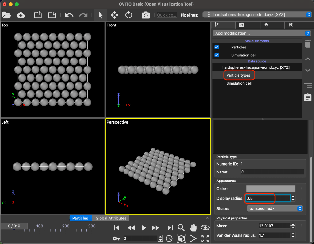
Then you’ll want to adjust the radius of the spheres / particles a bit like in the following image:

Finally you’ll want to color code each particle using the psi-6 values by adding a “modification” called “Color coding” as indicated in the following image:

That’s it! I hope you enjoyed the read and maybe started tinkering yourself :-).

Recently I found a beautiful, although unphysical behavior when I was implementing the dynamics of elastic billiard balls (hard spheres in physics lingo). And the bug was not at all where I expected it to be. But since while debugging I did not find any resource helping me out with this, and I think there is a good general lesson to be learned, I thought I write it up.

Pretty images

Okay. Mindset we want to simulate balls flying around and bouncing off of things, with the total kinetic energy being conserved. There is nothing else acting on the balls. No gravity, no nada.

So. Have a look at the animation below. What do you see?

Well. This is how it should look like

Did you notice something? Well besides the boring flying straight and occasional bouncing.

You may not, it takes a bit of patience and keen eyes. Both of which I lost during the debugging and looking at many of those animations to try and understand the problem.

Hence the impatient route. Let’s just trace out all the trajectories. Note, this only is visually manageable for a few balls for a few time increments, learned this the hard way.

Trace plot of the first animation

Trace plot of the second animation

You see it now don’t ya? 🙂

In each trace plot each ball has its own curve in the x-y plane. The color of the curve indicates the time the ball was at that location, starting off blue turning green and finally yellow. Each change in trajectory of a ball is denoted with a small black dot.

Now we can easily see that in the first trace plot that there are a lot of dots of two curves very nearby. Those are orbiting balls! Side note: THIS is how you keep sane analyzing those trajectories.

Equipped with trace plots let’s run the simulation for longer, just because we can and it neatly underlines the difference between the buggy implementation and the correct (boring) one.

We actually see something that resembles coils in the buggy trace plot. Pretty, no?

Event Driven Molecular Dynamics

The above thing is also referred to as Event Driven Molecular Dynamics (e.g. here). Juuust in case you want to research yourself a bit. Helps greatly to know the name of the things when researching.

When you have hard spheres without any external field, you are in the lucky position that you can just solve the equations of motion and jump the entire ball setup forward to the next event, instead of having to increment time by a small constant amount, hoping your time increment is small enough to not screw you over with numerical errors. The latter is the norm for molecular dynamics.

So event driven molecular dynamics works because hard spheres are totally unrealistic :P. I say unrealistic because normally you would expect that some effect applies between the balls which depends on their distance in some continuous fashion, like gravity or electro dynamics or what have you. Anyway.

The bug

The bug snuck in when implementing the estimate when the next ball-ball collision will be. It did because I copied the solution I found in a book, a paper and also on this page. Maybe I wasn’t paying close enough attention or something, but it still happened, so it may happen to you ^^. It was not, as I thought for too long, the numerical side, e.g. rounding errors.

This caused my bug

Δt is our time increment, Δv is the difference in velocity between our balls of interest, Δr the difference in their position and d = (Δv *Δr)^2 – (Δv * Δv) (Δr * Δr – 4 * sigma^2), for a prettier version see the same page again immediately below Δt definition I copied. sigma is the radius of each ball.

Do you see the bug? If so I congratulate you. I didn’t. So let’s step through it.

The Δt is derived from a single equation.

So a collision occurs once two balls are twice their radius, sigma, apart. The distance, Δr between their positions is

using balls k and l in two dimensions, that’s where the 1 and 2 indices come from. Both positions are a function of time like

So now all we have to do is go backwards and plug x(t) into our Δr equation and solve it for Δt. This coincidentally is a quadratic equation in Δt

with

Whose solution is ALMOST what had above. To prevent annoying scrolling, here it is again

it should be

with a +- sign and conditioned on the result being greater equal zero. By discarding the minus square root of d we ignore a second solution, which leads to some balls orbiting each other!!! So the original solution looks reasonable, but is technically not correct. Which was important here.

So what’s the general lesson I mentioned in the beginning?

Do use your intuition to understand solutions in papers and text books, but if you are implementing them try to understand the derivation of those solutions step by step. Otherwise you may end up orbiting bugs for some time. *ba dump tsss*

Tag: physics

Adventures in Hard Sphere Dynamics