Let’s continue our quest, started in the previous post, to classify individual atoms based on their surroundings. If atomistic simulations are foreign to you I recommend checking out this wiki article to get an idea of what I am talking about.
This post is probably a bit atomistic simulationy technical, but don’t worry if not all aspect become perfectly clear. The main message is that that for crystals one can use machine learning to discover useful classes without the need for painstaking prior labelling. The rest of this post just goes a bit more into detail of the required bits of machinery to achieve this discovery of classes.
1. Recap: Trajectories
In this post I will use the term “trajectories” throughout, with the same meaning as in the previous post. To briefly recapitulate I have put the schematic below.
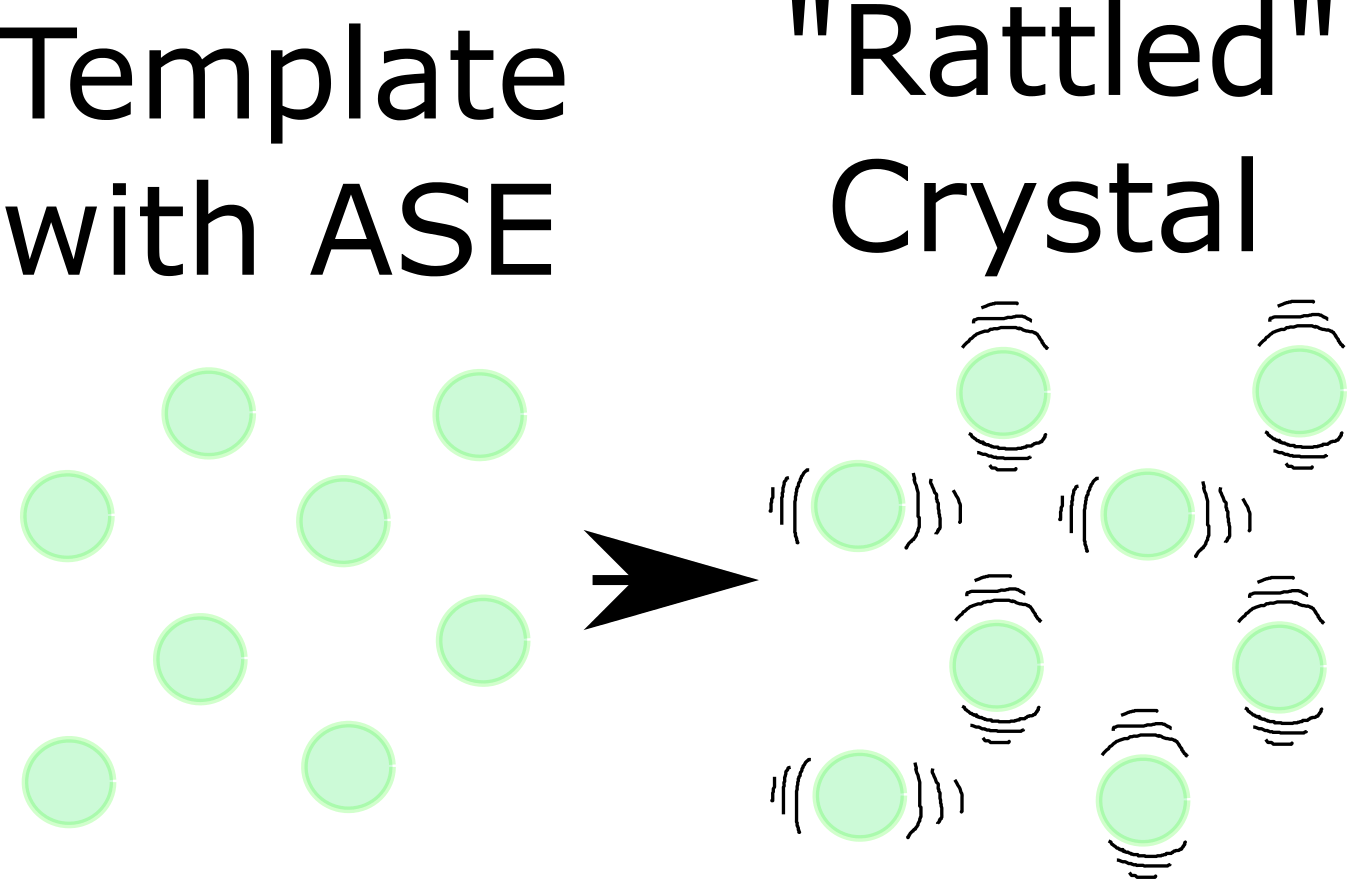
This schematic illustrates an ideal / template crystal, generated with the ase Python package, on the left. This template can be “rattled” (e.g. using molecular dynamics, Monte Carlo, using random numbers as done here, …) generating a new, slightly different, version of the original crystal. Perturbing the original crystal this way a bunch of times, possibly with different severities, leads to a collection of structures for one kind of crystal. This collection of structures for one kind crystal is what I will refer in this post as “trajectory”. So, it has a broader meaning than for molecular dynamics alone where it represents a series of snapshots of a crystal evolving over time.
If visualizing atoms in 3D is foreign to you, you can think of each perturbed crystal as a spreadsheet with each atom occupying one row and the columns containing x, y, z coordinates and other useful information. Then the trajectory of one kind of crystal is simply a stack of those spreadsheets. When we have multiple kinds of crystals we get multiple stacks like these.
2. Intro and Motivation
In the previous post we went through how to generate classifiers for individual atoms in a supervised learning setting. So, we claimed to know exactly which label is appropriate for which atom, to be able to teach the algorithm to distinguish atoms. However, in practise these labels are not always known for all atoms. Bummer! So, we need an algorithm which kind of achieves an understanding of the data itself. Algorithms of this sort are referred to as “unsupervised learning” algorithms.
In case you are unfamiliar with the supervised and unsupervised learning, you could imagine supervised learning as giving a kid a set of toys and while it is playing with it you are present and telling it what you want it to do with them (in this case the kid is the algorithm). Not being present and not telling the kid what to do with the toys and just letting it discover would then be unsupervised learning.
When we developed classifiers in the previous post we just threw in all the atoms we had for all structures into our training set and instructed the algorithms to find a way of distinguishing between those atoms, by the labels given to the atoms, to learn to make accurate predictions.
However, by throwing in all of the atoms, we discarded one very useful piece of information, that is which “trajectories” the atoms came from.
The kind of unsupervised learning I focus on in this post is based on approximating the distributions of atoms in feature space for each trajectory and decomposing those distributions (feature space = space spanned by selected properties of the atom, may not include spatial positions, see previous post). Sounds possibly difficult and convoluted but it is actually not as bad and definitively worth doing. But more on the details later.
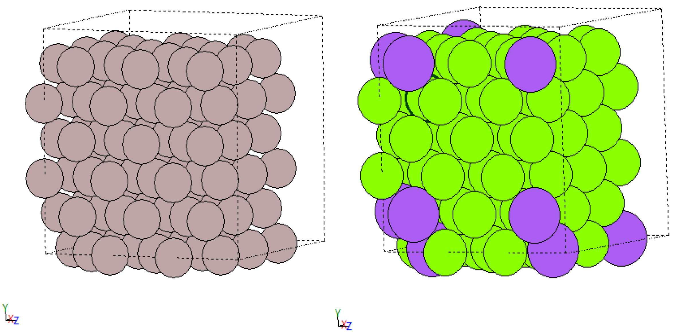
Let’s first have a look what this could be good for. The figure below is the result of the decomposition approach. In this particular case below a defect / a “vacancy” (missing atom) is present in the crystal and the decomposition algorithm identified two classes “vacancy-adjacent” and “pure fcc”.
fcc_vacancy_merged
Neat, no? In case you are underwhelmed let me point out that vacancies may not be the most exciting defects, but more materials sciency interesting ones become a lot less easy to explain in a brief form. The exciting part about the predictions in the image above is the small amount of work required for labelling (0!) with this approach to get useful classes. Really all I had to do was: i) throw in two trajectories one with a vacancy defect and one without, ii) choose my features (Steinhardt parameters [1] as in the previous post) to compute and iii) let the algorithm work it out.
So, in case you actually do atomistic simulations (if not don’t be afraid they are not that hard, check out this tutorial) and have trajectories you would like to analyse, all you would have to do is to: pick the features you want to compute, select your trajectories of interest and some other trajectories containing things you are sure appear in your trajectories of interest, e.g. certain lattice types, and throw all of those into the decomposition algorithm and it should be able to provide you with some useful classes.
So, this unsupervised learning approach ingests feature distributions (one per trajectory) and spits out distributions of characteristic effects. The meaning of the resulting distributions still needs to be determined by the user but is usually not too hard as seen in the vacancy example.
To get to those classes / distributions of characteristic effects used in the figure above I used two things: probabilistic mixture models and an algorithm for their decomposition. But to maximise clarity we will start the discussion simple by introducing first the decomposition idea in more detail, then discussing the K-Means algorithm and how to use if for trajectories. Then we will combine both and subsequently replace K-Means with the Gaussian mixture models (GMMs), one kind of probabilistic mixture model. Hence the post is structured as follows:
- the decomposition idea,
- testing the decomposition idea using K-Means,
- replacing K-Means with GMMs,
- studying defects in fcc crystals,
- some summarizing comments, and
- the three notebooks created for this post.
Before we actually get to the defects dataset we will use dataset from the previous post, where we can reasonably claim to be know all the labels. This way we can sanity check the output of our unsupervised learning algorithm (it is difficult to compute a classification score if the label is unknown).
3. The Decomposition Idea
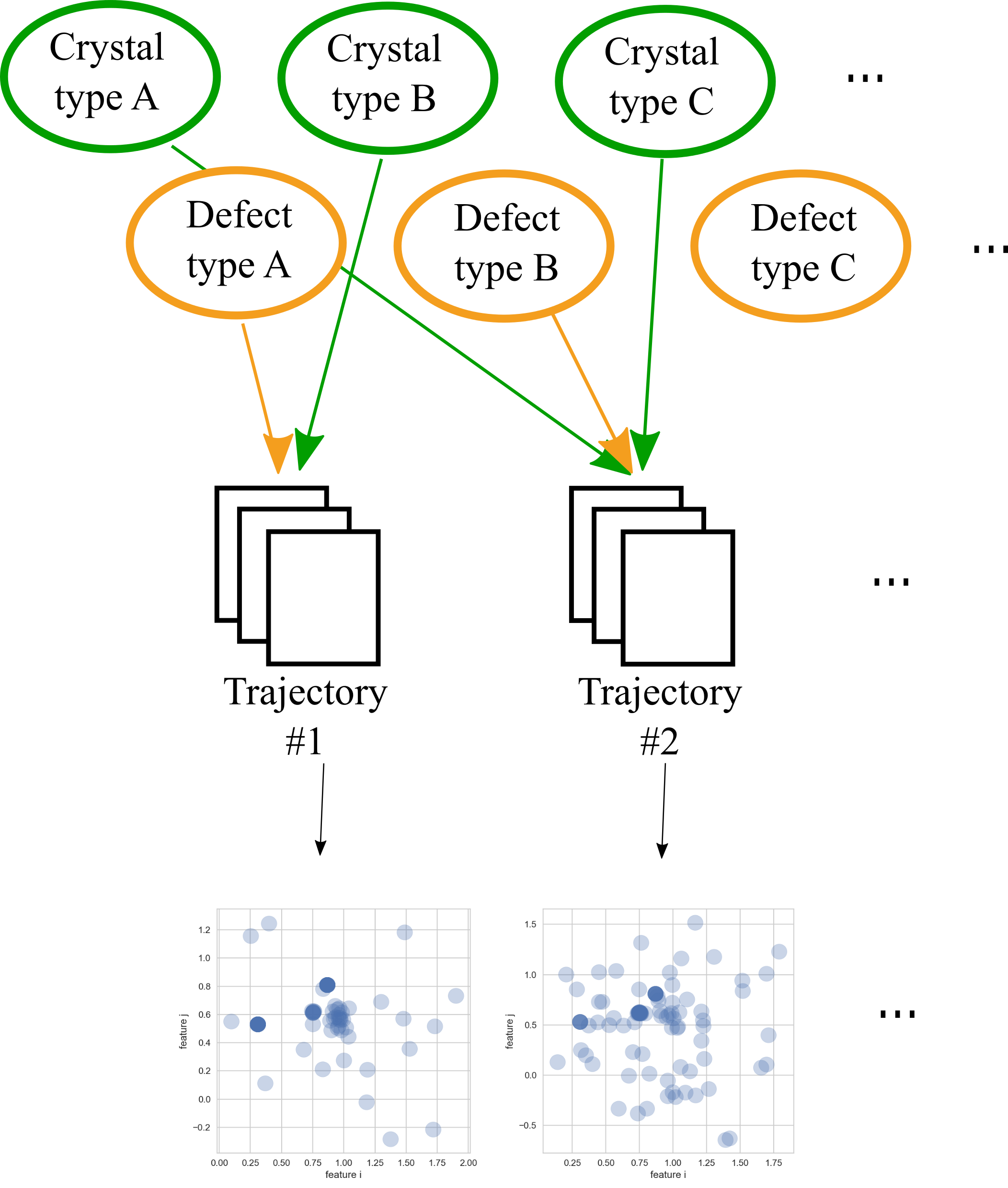
Let’s try to get a better understanding of the decomposition idea. For this I have created the schematic below. There the stacks of “spreadsheets” represent trajectories as discussed earlier.
Computing features for the atoms and taking two of those computed features for each atom we can plot all atoms in 2D, resulting usually in distributions much like those shown in the bottom of the schematic. So, each trajectory can be viewed as a distribution in feature space. This is nothing really new, we saw this also in the previous post. But comparing both scatter plots below we notice that at least one of the peaks seems to be roughly the same in both plots. This is actually something you can observe using for real simulated crystals, at least using Steinhardt parameters. So, we will make use of that.
decomposition_schematic
You probably noticed that I have omitted to mention the green and orange blobs at the top of the schematic, which is exactly what we have done assigning one label to an entire trajectory, we have just assumed one label per trajectory is perfectly fine. Those blobs represent characteristic effects such as type of crystal or defect. Normally each simulation is made up of a couple of these characteristic effects and you rarely have only one effect, say a pure fcc (face centred cubic) crystal, in an entire trajectory.
So, let’s think about analysing the distributions in feature space themselves. If you have a decent set of features it is fair to assume that each characteristic will cause a somewhat similar distribution in any trajectory, just as in our schematic above. Therefore, any distribution of a complete trajectory would be a superposition of distributions of characteristic effects. Hence, our new objective could be to try to represent the distributions of trajectories as adequately as possible using analytical approximations. Then breaking those approximations down into the smallest reasonable chunks. These chunks would then ideally represent those green and orange blobs in the schematic.
The next question then is how to break those approximations into chunks exactly, more on that in K-Means bit.
Generally, what those chunks mean also remains then to be determined, but it helps to take a structure where those are frequent and plot that structure highlighting the atoms of that chunk of the distribution. So that’s not too hard.
4. K-Means and the Decomposition of Trajectories
Becoming more concrete, let’s use K-Means as our analytic approximation of the distributions in feature space. This is somewhat crude, but I think is a very useful first approximation to understand how the decomposition idea works. The idea is pretty much the same for GMMs, just the technical side changes a bit.
4.2 What is K-Means?
Given a list of points (the dataset) in some space and a fixed number of cluster positions (centroids) the algorithm tries to find optimal cluster positions and follows this procedure:
- Initialize the centroid positions,
- Assign data points to the closest centroid (hard assignment),
- Recompute centroids using assigned data points and,
- Repeat from 2. until the end of time or a more useful criterion is reached.
For example, modifying the sklearn example for 2D, K-Means looks something like in the plot below. The colours indicate the cluster assignment.
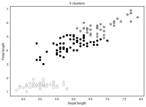
KMeans_sklearn_example
Since our data comes in bunches / trajectories it makes sense to use K-Means in two ways: i) fitting the data from all the trajectories “simultaneously” (as above) and ii) fitting the data for each trajectory “individually” and then use those models somehow.
Hence in case i) each cluster is supposed to represent some useful effect. Classification then proceeds by checking which centroid is the nearest centroid for a new point in feature space. Case ii) is fiddlier. I have implemented it such that the classifier stores one set of centroids for each fitted trajectory (later those will be decomposed) and analyses which trajectory has the closest centroid to the new point to be classified and uses the label for that trajectory.
Since we will decompose those sets of centroids obtained for each trajectory by default, let’s refer to each set of centroids stored as “model”.
But before using trajectories from actual crystals let’s “synthesize” some data and throw both of our K-Means classifiers at it.
Let’s assume we have three trajectories we want to find underlying models for and let’s assume we compute 2 features for each atom. The feature space distributions for the faked trajectories are shown on the right in the figure below, indicating the trajectories by colour. There you see that trajectory 1 and 2 seem to contain the same characteristic effect.
KMeans_allatonce
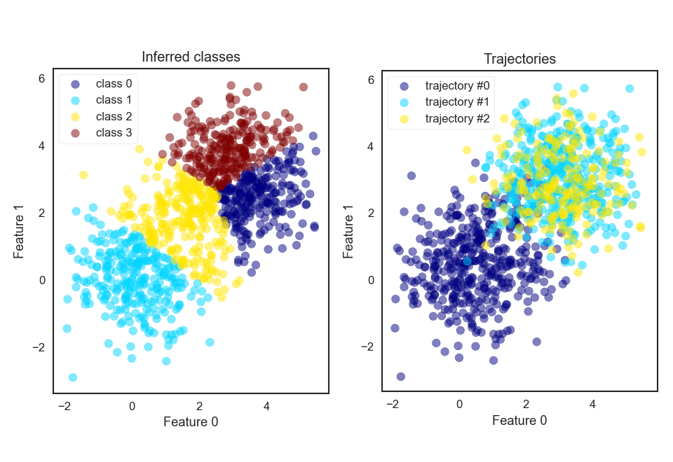
Now let’s see how the “simultaneous” and “individual” K-Means versions do using 4 centroids.
One the left of the figure above the atoms are coloured using the “simultaneous” K-Means classifier. So far so meh. See how the plot on the left doesn’t really correspond to one of the right in terms of coloured dots?
Now, if we use the “individual” method, and make use of the decomposition algorithm we find K-Means models, as shown on the left in the next figure, which more closely resembles what we would expect (two models where each model contains one of the two blobs). Instead of finding two inferred models, one for each big blob we find that one big blog is shared by three models. But that is also fine. In practise you would look at the classified atomic structures and realise that all three classes belong to the same effect and just combine them for further evaluation. Alternatively, you could tweak at the knobs of the decomposition algorithm or underlying algorithm, such as K-Means.
KMeans_sequentially
How does the decomposition algorithm work in the context of K-Means, you ask?
The decomposition algorithm first pre-processes the models by checking each K-Means model (model = set of centroids) obtained (one model per trajectory), computing the similarity of all components (centroids). Similar components are replaced, e.g. by an averaged version, and added to a library of components. Components which are unlike all other are added to the library as well of course. The resulting models then consist of combinations of those components stored in the library. Then the models are decomposed by comparison, for which there are four cases:
- two models are identical (e.g. same type of crystal in more than one trajectory),
- two models share at least one component but not all (e.g. both trajectories share some type of crystal but also contain different ones),
- one model is a subset of another model (e.g. one trajectory contains one type of crystal which is also found in another model, among other types) and,
- two models share no components.
Because the algorithm works on a library of components it only needs to deal with integers representing those components. So, the algorithm loops through those sets of integers using set operations, which itself is very fast.
This algorithm does not become much more complicated for mixture models, since they also contain component positions / centroids.
4.2 K-Means over all trajectories simultaneously
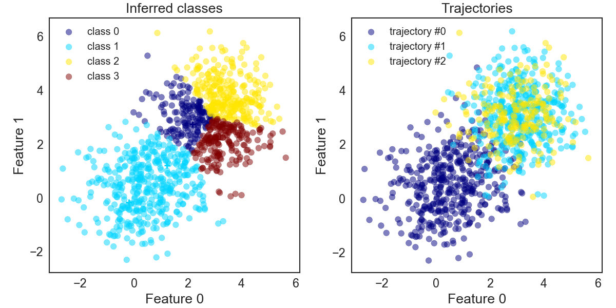
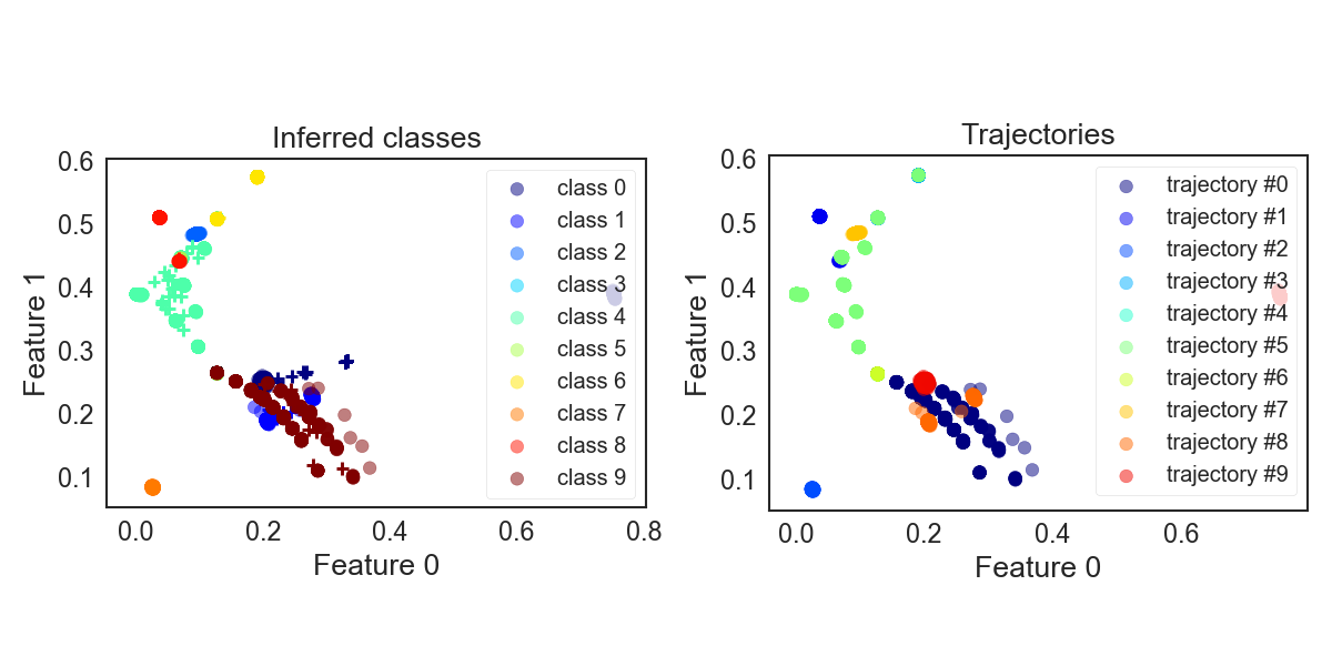
Now that we have an idea of how the decomposition algorithm works with K-Means, let’s compare the “simultaneous” and “individual” K-Means versions (the decomposition algorithm is part of the latter). For this let’s use the dataset of the previous blog containing a variety of crystals. Those crystals are quite different, so decomposition itself is not expected to do much, but let’s see if there is a difference in using the “simultaneous” and “individual” versions of K-Means.
The figure below shows the true distributions of the trajectories, colouring by crystal type. On the left side the atoms are coloured by their predicted label. Without having to look too carefully one can see that this doesn’t seem to work too well since the clusters receiving the same colour are quite different to the true groupings. So far so meh.
KMeans_crystals_allatonce
Assume that the K-Means find the same centroids for every execution, even then their numbering, and thus the labels the classifier assigns, will differ. This identification problem of which model label corresponds to which type of crystal also appears for the following methods.
So, to get our hands on some accuracy scores let’s take the predicted class which is most frequent for one trajectory and designate it as the class for that trajectory (reasonable for this dataset, no?). Having identified which class belongs to which trajectory allows us to compute F1 scores (score of 0 = bad and score of 1 = good). The figure below shows that the accuracy for some crystals is very good whereas for others it is quite terrible. Meh, indeed. But no surprise there, assuming 10 centroids would magically be sufficient to classify 10 types of crystals is a tad naïve.
KMeans_crystals_allatonce_bars
4.3 K-Means over trajectories sequentially & the decomposition algorithm
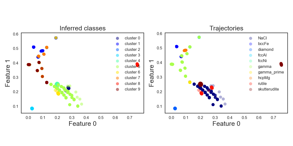
Now let’s take the “individual” K-Means approach. The distributions in feature space are shown in figure below. On the right side again coloured by crystal type. On the left side coloured by predicted label.
This, surprisingly, actually already does look quite good. You may be wondering why the colourings allow non-roundish shapes despite K-Means. This is because the plot actually is a projection onto 2D space and not a cross-section.
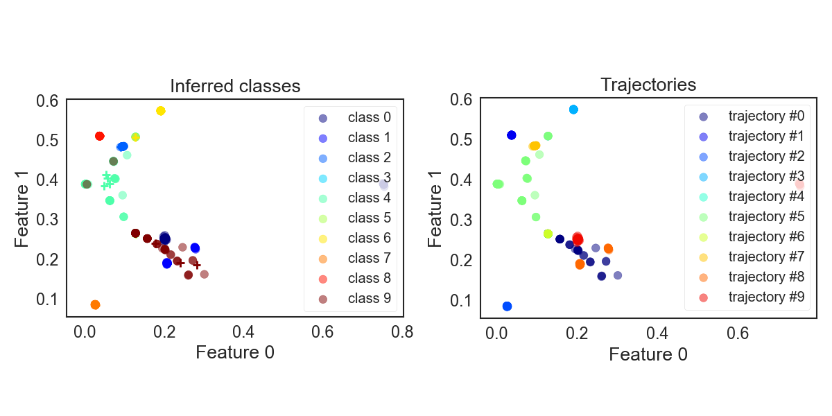
KMeans_crystals_sequentially
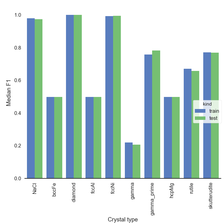
Computing the F1 score the same way as before, we get the below F1 score diagram. And whoa, the scores are much better than when fitting all the trajectories simultaneously. They are also quite good despite the very simplistic hard assignment of an atom to a cluster just by distance.
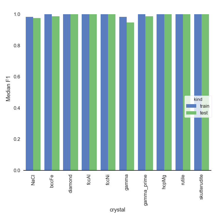
KMeans_crystals_sequentially_bars
I don’t know about you, but I was honestly surprised by this. But then the crystal types are quite different, and we are clustering in 9D space. At any rate, we definitively want to continue testing the “individual” approach.
5. Mixture Models
Now let’s replace K-Means with probabilistic mixture models.
5.1 What are Mixture Models?
One way to do better than hard assignments based on Euclidean distances in feature space is to use probabilities. Since a proper introduction of probabilistic models is beyond the scope of this post I want to refer you to wiki, or Christopher Bishop’s excellent Pattern Recognition and Machine Learning book.
Let’s use Gaussian mixture models (GMMs) as our probabilistic mixture model of choice. These are similar to K-Means in the sense that they place Gaussians / bell curves at the centroids. So, instead of using distances as a measure for the classifier directly, we go via Gaussian functions, which take the distance as input. One special property of Gaussians is that the area under their curve is finite. So, we can combine multiple Gaussians using weights, one per Gaussian. The kind of mixture we use here has all weights summing to one and the area under the curve of all the Gaussians are one.
What we want those mixture distributions to do is to approximate the frequency distributions, as for example shown in the figure below. There the crosses are atoms of all trajectories. The contour plots in 2D represent the frequency distribution of those atoms as a function of both axes X and Y. The curves with the shaded area along x and y are the frequency distribution along that axis only.
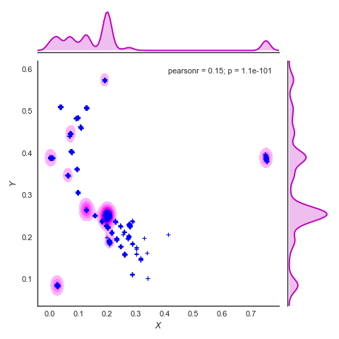
Density_plot
In principle we can use GMMs fitting the trajectories either “simultaneously” or “individually”. Since we have seen that the “individual” mode seems to do better for K-Means we will go with that.
Different to K-Means is that we need to re-adjust the weights for each GMM model after decomposition. Don’t worry, this is done under the hood by fitting the weights of each model, obtained after decomposition, to the complete data set.
5.2 Gaussian Mixture Models over trajectories individually
Adopting our “individual” modelling method to GMMs and classifying our atoms we get the resulting assignments below. Which seems pretty close to the reference.
GMM_crystals_noDirichlet
Computing the F1 score the same way as before seems to confirm this impression. The overall score seems to also be better than with K-Means, nice!
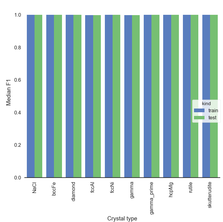
GMM_crystals_noDirichlet_bars
5.3 Comparison of K-Means and Mixture Models
So far so good. Now we know that GMMs seem to do better for our task of inferring robust classes than K-Means, both using the decomposition algorithm. But I haven’t mentioned how this does with varying dataset size. So, let’s get to it now.
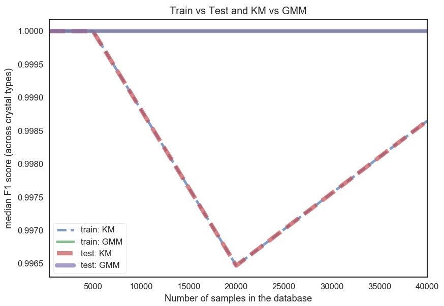
Selecting a couple of noise distributions for the rattling and varying the size of the dataset from 250 to 24,000 computing the median of the F1 scores over all crystals we get the plot below.
Comparison_plot
The dashed lines are the K-Means (KM) classifier. And we can see that it seems to fluctuate with increasing dataset size, unlike the GMM classifier. Also, both test and training curves overlap perfectly for each classifier. That training and test curve overlap so strongly is likely because the training and test set are results of splits of the entire dataset (for the respective dataset size) randomly choosing out of all structures. This would probably be different if the split would be done over structures themselves. That the KM curves wobble unlike the GMM curves could be due to the isotropic nature of K-Means in this case (due to the distance condition). GMMs on the other hand are fitted with full covariance matrices for each component and more flexible (means they can become ellipsoidal). But all in all, both KM and GMM lead to quite decent F1 scores across all dataset sizes.
6. Application of Mixture Models to Defects
Now, having done our homework, we can apply the decomposition algorithm to a more interesting task. I have chosen one task here where I was interested in seeing if, by comparing trajectories with fcc only, fcc + a vanacy and fcc + symmetric twin grain boundary, our approach could develop distinct classes.
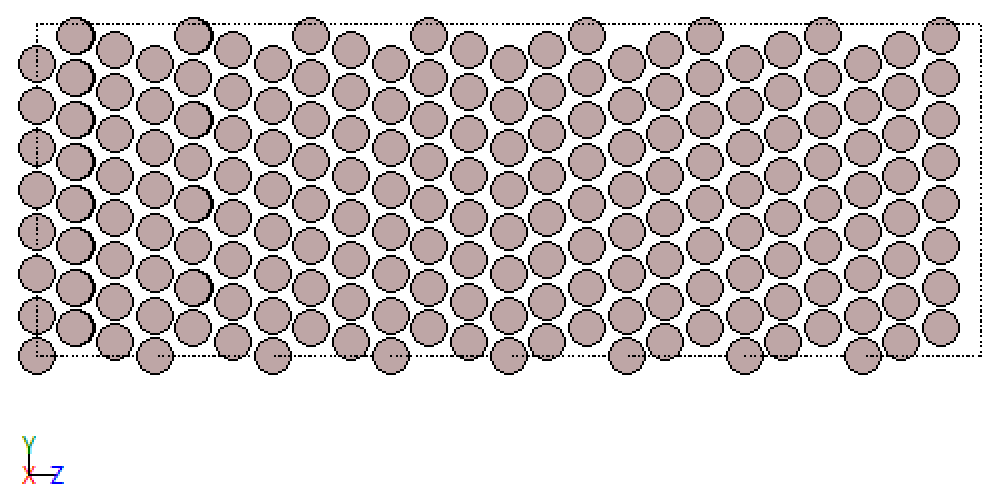
You have already seen earlier that this approach works for vacancies, but so you don’t have to scroll and because I think it’s very pretty you can see it again below (left image before classification and right image after classification varying circle size and colour by predicted class). So, we actually found a class for the vacancy!
fcc_vacancy_merged
Similarly, we find a class for the atoms in the twin grain boundary. Below you see the crystal before and after classification. Note, while each class receives its unique colour for the classified plots the choice of colour relative to the unclassified structures is quite random.
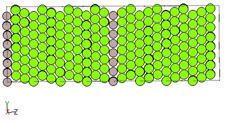
fcc_Sig3GB_GMM
This is neat. So, the decomposition algorithm allows us to study the grain boundary and the defect, with relatively little effort on our side to dive into the weirdness of grain boundaries. This approach also works for other grain boundaries. If that’s not donkey balls!
7. Summarizing Comments
Summarizing, we managed to slightly modify pre-existing unsupervised learning algorithms to do laborious work for us and discover classes for atoms, allowing us to generate pretty pictures. Aside from generating pretty pictures this method could be quite useful in a variety of ways. Of particular interest could be the tracking of defects over time or the identification of phase transitions. You could also use it for any problems where you would want to use classification but can’t come up with the labelling yourself (at least for atomistic structures).
Additionally, to the two discussed modes of fitting trajectories “individually” or “simultaneously” one could also imagine a third, “hierarchical”, version. For this version all model components could explicitly be shared while fitting each trajectory individually. This would prevent the step of having to compare components after the individual fitting as done here.
I have played around trying to implement this hierarchical approach with pymc3 but I did not see how this could be done in a way such that it would really scale beyond 1D to the present case, where we have tens of thousands of data points or more for half a dozen trajectories or more. At any rate, I have added my attempt for a simple 2D case below. If you have any ideas, let me know!
That’s it!
Thank you for reading this post, I hope it was interesting, entertaining or even useful. If you like it leave a comment or forward this post to a friend.
See you next time when I’ll probably write about predicting electron densities of atomistic models.
Literature
[1] P.J. Steinhardt, D.R. Nelson, M. Ronchetti, Bond-orientational order in liquids and glasses, Phys. Rev. B. 28 (1983) 784–805. doi:10.1103/PhysRevB.28.784.
8. The Notebooks
8.1 K-Means + GMMs for crystals with known labels
Notebook covering everything until and including section 5 (in that notebook you’ll want to replace the path the the atomtoolbox package):
8.2 K-Means + GMMs for crystals with unknown labels using decomposition of distributions
Notebook covering section 6 (in that notebook you’ll want to replace the path the the atomtoolbox package):
Notebook containing the toy example for the hierarchical approach using pymc3: