In this blog post I will show you how freely available machine learning tools (scikit-learn and tensorflow) in Python can be used to solve a non-trivial task, the classification of individual atoms in some complex arrangement of atoms. The jupyter notebook used here can be found at the end of this post. The aim of this blog post is to give you an insight in how classifiers for atoms can be created and tested and to enable you to create and test your own, using a selection of types of crystals of interest to you.

This post is structured as follows: Initially, I will outline what I mean by ‘classification’ (section 1), then you get to see real atoms (well pictures of real atoms, see section 2) and imaginary simulated atoms, followed by the characterization of ‘mobs’ of atoms (section 3), then we get into how to train your computer to perform the trick of classification (section 4) and lastly we will use our trained classifiers to make predictions (section 5) and study an until then (in the training) unseen type of crystal. Classifying the unseen type of crystal will demonstrate what surprising contributions trained classifiers can make to the analysis of crystals.

1. Crash course in classification

Classification, in general, is the process of taking some input information for some object and assigning it one of a couple of possible labels, for example looking at your watch in the morning (the input is your visual of your watch) and deciding it’s too early to get up (“too early” and “wow, I better get up” are your seemingly only possible two labels, no?). In this instance it is fine to perform the classification manually since you will only have to check one watch and are doing so perhaps only once every 15 minutes. But you can imagine checking more watches every few seconds or less may be quite strenuous.

When you see your watch and decide to get up or not, you use a wonderfully complex classification algorithm located in your brain, which uses your experience up to this point and your understanding of the world you are in, to guess which label to assign. An approach to emulate this with your computer is to provide it with a database of times and tell it which label belongs to which time as in the table below (the labels appeared magically form somewhere).

Time [HH:MM]	Label
04:15	“too early”
08:21	“wow, I better get up”
12:43	“wow, I better get up”
…	…

So, you explicitly tell the computer the meaning of the given times and learns a statistical pattern between the input “Time” and output “Label”. This approach is referred to as supervised learning.

The analysis of atoms is not much different from the watch example, we only consider different objects and assign different labels. So instead of looking at watches we study usually many thousands of atoms which move about over time. But imagine looking at 100,000 or 1,000,000 watches… How far do you think you would get before soundly falling asleep?

So, we definitively want to automate this process. But you may ask, what information, also referred to as ‘features’, our decision for a label would be based on? Could it be the number of atoms within a certain distance? Or what about angles? But what if we decide to look at the crystal from a different direction, the crystal doesn’t change but do our features? You see this is a non-trivial problem, one which has been pondered by quite a few people over the last decades and is still being worked on.

One of the reasons why features are still being researched is that the choice of representation is also influenced by the goal, i.e. which kinds of labels you want to be able to assign to atoms. Because, depending on how specialized that label is, the features must contain the necessary information. For example, the time on your watch itself contains insufficient information about the slipperiness of your shower.

Generally, we will use some representation of how the neighbouring atoms are configured relative to the atom of interest. We will get into those features a bit more in section 3.

Similarly, to our list of times and labels “too early” and “wow, I better get up” we need to get some crystal data and labels from somewhere to create our classifier. Luckily, we can make use of the great atomistic simulation environment package (a Python package). In the notebook I used that package to create a bunch of crystals types as templates. Creating crystals this way from scratch has the advantage that we know which label the atoms should receive so we can apply algorithms of the supervised approach. To multiply the size of our database (more is usually better) crystals will be perturbed as in the figure below, but more on that later.

Except for three specific types of crystals (‘gamma’, ‘fccNi’ and ‘gamma_prime’) the others are chosen quite arbitrarily. I will discuss these three ominous crystals a bit more in section 5, where one of the trained classifiers is chosen to analyse an, till that point, even more ominous and unseen crystal. But before we disappear in the lofty heights of how to train our computer to do tricks with atoms let’s look at what atoms look like in the non-simulated physical world. Wasn’t there some physicist who proclaimed if experiments don’t agree with theory they are wrong or so?

2. Can you even see individual atoms?

It turns out, yes, you can, under certain conditions. Below in Figure 3 is an image of a 2D structure with greyish and black blobs. The greyish blobs are atoms as seen under an electron microscope, which is a microscope which uses electrons instead of light (rad, isn’t it?). The black blobs are the space between atoms.

Not yet quite atomic scale but still very pretty microscopy pictures can be seen here  (beware, there may be some bugs). There is also a neat video by the nature journal here showing an atomistic reconstruction of a 3D nanoparticle of a crystal.

To illustrate the type of magnification required to make individual atoms visible, assume that the white blob representing a nitrogen atom is approximately 1 cm across in the image. The actual atom itself has a covalent radius of 71 pm. This is 9 to 10 orders of magnitude difference! For comparison, that’s the same order of magnitude difference between the kinetic energy of a small apple falling 1 meter in Earth’s gravity against the kinetic energy of an airbus A380 at cruising speed!

Besides registering that there are blobs, electron microscopes can also identify which kind of element or chemical species a registered atom has. Which brings it close to the information one normally sees in visualizations of simulations of atoms which we are here interested in. An example of such a picture of simulated atoms is shown in Figure 4. There we see a diamond crystal from a certain angle to make a pretty hexagonal pattern of atoms. The colour indicates the element, in this case Carbon. In other example more than one colour will appear, indicating the presence of more than one element.

3. How to characterize individual atoms in a ‘mob’ of atoms?

To develop any features for the classification of an atom, we take information from the local neighbourhood of that atom. Let’s call that collection of atoms a ‘mob’. Let’s also refer to the atom we use to construct the mob around as the mob’s central atom. The conditions under which the mob is commonly chosen are based on the distance in 3D Euclidean space. After sorting of the neighbouring atoms in the crystal with increasing distance one can, for example, choose some fix number of nearest neighbours or all neighbours within some cut-off radius. The mob is then defined for each atom by choosing one of those two conditions.

If the crystal is part of some simulation, e.g. molecular dynamics of Monte Carlo then we determine that mob for each iteration anew. This could also be done, in principle, using information from experiment, if there weren’t some pesky issues with the resolution and destructiveness of the current methods.

Having identified the mobs, we want to compute features. Here we will focus on one particular kind of feature extracted from those mobs, the so-called bond order parameters, see Steinhardt et al. [1] for detailed information. Generally, bond order parameters use spherical harmonics (special kind of function) to extract information from each atom’s mob bond geometries. These bonds can be imagined as lines, as in the figure below, from the mob’s central atom (red dot) and all atoms in the mob (pink dots). These lines or geometric bonds (since not necessarily chemical bonds) define the bond geometry of one mob. Now imagine drawing a sphere around that central atom (the black circle around the red dot). Marking where each geometric bond crosses this unit sphere (indicated by blue hatches) results in a distribution of blue hatches on the sphere.

This distribution of blue hatches itself can then be approximated using spherical harmonics, similarly as time dependent signals can be approximated using the sine and cosine functions. Bond order parameters use this approximation to give values which do not change when the reference coordinate system is translated or rotated, which is just very useful. You don’t really want features for classification which tell you a different story depending on from where you look at the crystal, since this really is more information about you and not information about the crystal.

Bond order parameters also allow the very useful distinction of very common types of crystals (very handy for our example at the end). Note that, generally, we could use all sorts of kinds of features and are not limited to a single kind like bond order parameters to train classifiers. If possible, you should always use as many features for your classifiers as you reasonably can.

For an overview over features for different kinds of arrangements of atoms, organic and inorganic structures see Keys et al. [2] (also has excellent graphical representations). For a review of features for metals and alloys with crystal defects see the excellent paper of Stukowski [3]. Another great review of features with the focus on artificial neural networks is given by Behler [4].

Here we use a slight modification of the bond order parameters, making them somewhat sensitive to the chemical information available, besides the local bond geometries. That is, we compute three version of each bond order parameter using different ‘filters’ as used by Schmidt et al. [5]: using all the mob’s atoms, i.e. the ‘all’ filter; using only those of the mob’s atoms whose chemical species is like the central atom’s species, i.e. the ‘like’ filter; and using only those of the mob’s atoms whose chemical species is unlike the central atom’s species, i.e. the ‘unlike’ filter. This will allow us to differentiate between geometrically identical crystals whose sole difference is the placement of specific elements.

In Figure 7 the distributions of one of those bond order parameters is shown for all the types of crystals contained in our training set: NaCl, bcc Fe, Diamond, fcc Al, fcc Ni, gamma, gamma_prime, hcp Mg, Rutile, and Skutterudite. If you don’t know those crystals don’t worry. In the jupyter notebook is a cell you can use to visualize each of those to get familiar.

 

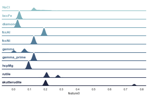
To generate this database visualized in Figure 7 each type of crystal was created in its ideal form as a template and then ‘rattled’ with forces of different magnitudes. This rattling can be done in different ways, e.g. you can run a molecular dynamics simulation at some temperature and pressure and use the observed configurations which change over simulated time or, as done here, you select a couple of distributions from which you draw random displacements for each atom and apply those. With increasing width of those distributions, the atoms are increasingly displaced, emulating the effect of temperature minus the general expansion of the underlying lattice. This ‘rattling’ to multiply the database of course assumes that the type of crystal remains unchanged.

In case you want to also use this as a shortcut for your simulations be aware that the features you compute may depend on the expansion of the crystal in all directions, which may not be the same, i.e. expansion in one axis may be slower than along the other two leading to a different evolution of your feature values than an equal expansion. At any rate, drawing random displacements is quite cheap and can yield useful classifiers. The distributions in Figure 7 were generated using 6 Gaussian displacement distributions with variances ranging from 0.001 to 0.03 Å and mean zero. For each of those distributions, displacements were drawn 20 times and applied (not cumulatively) to the ideal crystal templates.

Then for each of those rattled configurations the bond order parameters were computed for all mobs using a fix cut-off radius of 4 Å. You can see in Figure 7 that quite different distributions emerge, depending on the crystal type. If, instead of a cut-off radius, we would have fixed the number of neighbours for the construction of the mobs to say 12, the ‘fcc’ based crystals would have shown identical distributions disregarding the chemical species of the atoms. With a cut-off radius the distributions of feature0 are different because of each type of crystal is defined with a different lattice constant.

So, evaluating classes based on one feature seems quite doable, but what if we have a couple of those? Suddenly that’s not really something we can easily visualize anymore. Hence our next strep is to train classifiers and evaluate their worth. Then we are all set to study the unseen crystal.

4. How can we make use of those pretty distributions?

One case of classification, is if we have only two classes. In this case one speaks of a binary classification problem (very descriptive, no?). An example for this kind of classification algorithm is the famous support vector machine, a maximum margin classifier, which tries to identify so-called decision boundaries in the space spanned by our features to make the least classification errors.

However, we are here dealing with more than two classes of crystals. For this we can still use binary classifiers, either by developing as many classifiers as there are unique class combinations (that number can explode terribly) and then let them vote or develop classifiers to distinguish between the class of interest and the ‘rest’. These two approaches are also called ‘One versus One’ (OvO) and ‘One versus Rest’ (OvR). Beyond binary classifiers there are, for example, neural nets (using the softmax function), decision trees and naïve Bayes. One could decide to use only one of those to develop a classifier, and if I would have to implement them from scratch that’s probably what would I have done. However, others have been so kind to do the work and make those algorithms available, so we can just test all of the mentioned algorithms and more. The notebook contains a series of algorithms for comparison. Each algorithm requires the fiddling of specific knobs aka ‘tuning of hyperparameters’. This is done in the notebook using scikit-learn’s GridSearchCV class, at least to a degree to set you up for more serious refinements.

But before that the atoms and their feature vectors are sampled from the database to generate new stratified databases (stratified = equal representation of each class) of 21, 42, 100, 500, 200, and 6000 samples/atoms per class, to test convergence of the algorithms with database size. Before the training of the classifier commences these stratified databases also split into test and train set with a 40% – 60% split. This is to test the overfitting / generalizability of the trained classifiers.

In total there are 9 features in this example, 2 of which are used to visualize the sections in feature space which are associated with individual classes, as shown in Figure 8 and Figure 9 for artificial neural network (ANN) and decision tree based classifiers (note that ANN here is created using scikit-learn’s MLPClassifier whereas DNN appearing later is also deep artificial neural network created with a custom class based on tensorflow). The dots with delicate white borders indicate individual atoms of different crystals (same colourmap as the colour bar on the right). One can clearly see that different algorithms definitively partition space in quite different ways.

A common method to verify the quality of a binary classifier is the Receiver Operating Characteristic (ROC) curve. This curve plots the ‘true positive rate’ against the ‘false positive rate’. In this case we deal with multiple classes, but one can compute the ROC in OvR fashion for each type of crystal and see how the classifier fare. Results of this are shown as an example for naïve Bayes in Figure 10, training the classifier on the 500 samples per class database. For comparison, a classifier which would label uniformly at random would lead to a straight diagonal curve from the bottom left to the top right in Figure 10. We get ROC curves some of which follow first the y-axis and then the x-axis closely for some crystals and less closely for others, indicating a variation in the naïve Bayes classifier’s quality depending on the crystal type. Also, each crystal is represented twice by the results for the test set and for the training set in form green and blue lines respectively.

A quantity derived from the ROC curve is its Area Under the Curve (AUC), also referred to as ROC AUC. Consequently, an ROC AUC close to one is one indication of a good classifier. Note that there are quite a few metrics available as well. To compare the different trained classifiers and the difference of their predictions over test and training data, the classifiers ROC AUC values are plotted as a function of the number of draws from the stratified database in Figure 11 for the ‘gamma’ crystal. I chose the gamma crystal because it is chemically disordered version the ‘gamma_prime’ crystal, as shown further below. Thus, the possible confusion of the classifiers is quite high. We see that the ROC AUC values seem to mostly stay above 0.95 anyways without significant worsening with increased number of drawn samples.

To give a better overview over how the classifiers fare regarding the crystal type, each classifier’s ‘precision’ or ‘true positive rate’ times 100 is shown in dependence of the crystal type. One can see that most classifiers seem to perform quite well, apart from AdaBoost.

5. Classifying an unseen structure

Lastly, let’s see how the classifiers perform on some combination of crystals which was not seen during the training. The new crystal places one type of crystal (‘gamma_prime’) in form of a sphere within another type of crystal (‘fccNi’), replacing that crystal’s atoms. An example of the ‘gamma_prime’ crystal is shown in Figure 13. As you can see it has circles with two colours, brownish and green representing Al and Ni respectively. The brown circles (actually spheres since originally 3D) are sitting in the corner sites of the underlying lattice (face centred cubic = fcc). The host crystal, ‘fccNi’, is shown in Figure 14. This, quite anticlimactically, differs from ‘gamma_prime’ by not having Al in the corner sites but Ni and by having a different lattice constant (in this case the distance between the two closest corner site atoms), although not visible in the image. This example is chosen because it is close to technical relevance for the simulation of real materials and because there is a neat surprise awaiting you.

If we apply, say, the ANN classifier and select all the atoms classified as gamma_prime for visualization we get a spherical structure as in Figure 15, which we expect. But wait, computing the percentages of identified classes in the crystal we get fccNi = 84.03%, gamma_prime = 9.83%, and gamma = 6.15%. How could this be without us inserting that phase in the first place?

Quickly plotting all atoms identified as gamma we find the structure in Figure 16 and find a spherical shell-like structure around the ‘gamma_prime’ sphere.

You may be surprised because if you place ‘gamma_prime’ in ‘fccNi’ you would expect a classifier who knows how the crystal was constructed to only use those two labels for all the contained atoms. However, our classifiers have no idea how we constructed the crystal and must base their predictions on the features we provide. Remember, our features of each atom are dependent on the surrounding mob of atoms. Hence sufficiently close to the interface of ‘fccNi’ and ‘gamma_prime’ neither of those classes really describes the mob of atoms observed. Although we globally see that there is an ordered to the shell, locally the mobs look much more like chemically disordered mobs as in the case of the gamma crystal, see Figure 17.

That’s it! Using the notebook below you should be able to reproduce the above and can go wild testing other types of crystals. The AtomToolBox package I used you can get here.

I hope you enjoyed the read! If you like it share it and or leave a comment.

In the next post I will discuss how unsupervised learning can be utilized to develop classifiers when your database contains crystals where not all atoms of a given crystal should be assigned the same label. This for example is the case when there are crystal defects, such as grain boundaries.

Eric

The notebook

Acknowledgements

Thank you, Andrew Fowler for reading through this post and your suggestions!

References

[1] P.J. Steinhardt, D.R. Nelson, M. Ronchetti, Bond-orientational order in liquids and glasses, Phys. Rev. B. 28 (1983) 784–805. doi:10.1103/PhysRevB.28.784.

[2] A.S. Keys, C.R. Iacovella, S.C. Glotzer, Characterizing complex particle morphologies through shape matching: Descriptors, applications, and algorithms, J. Comput. Phys. 230 (2011) 6438–6463. doi:10.1016/j.jcp.2011.04.017.

[3] A. Stukowski, Structure identification methods for atomistic simulations of crystalline materials, Model. Simul. Mater. Sci. Eng. 20 (2012) 45021. doi:10.1088/0965-0393/20/4/045021.

[4] J. Behler, Constructing high-dimensional neural network potentials: A tutorial review, Int. J. Quantum Chem. 115 (2015) 1032–1050. doi:10.1002/qua.24890.

[5] E. Schmidt, P.D. Bristowe, Identifying early stage precipitation in large-scale atomistic simulations of superalloys, Model. Simul. Mater. Sci. Eng. 25 (2017) 35005. doi:10.1088/1361-651X/aa5c53.